The idea: every node knows how big its subtree is
A binary search tree finds a key in one root-to-leaf path. It cannot, by itself, answer “what is the 7th smallest key?” or “how many keys are smaller than 66?” without walking the keys in order, which is O(n). An order-statistic tree adds one number to every node: size, the number of keys in the node's subtree, itself included.
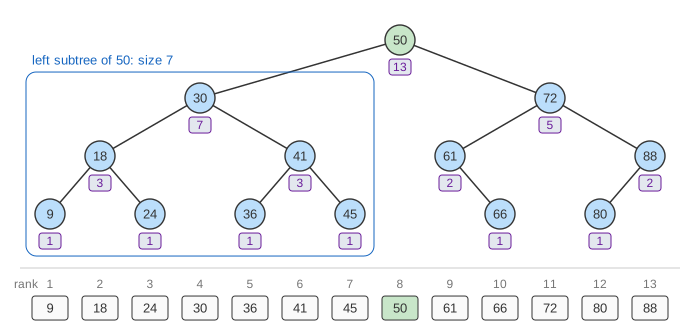
The sizes obey one rule, size(x) = size(x.left) + size(x.right) + 1, and an empty subtree has size 0. From it follows the key fact: inside x's own subtree, x is number r = size(x.left) + 1 in sorted order. On the page each node's size is the purple box under it, and the nodes are drawn at their in-order positions, so the sorted row at the bottom lines up with them: a key's rank is its column.
Select(k): the k-th smallest key
select(x, k):                 // k-th smallest in x's subtree
    r = size(x.left) + 1
    if k == r: return x
    if k < r:  return select(x.left, k)
    else:      return select(x.right, k - r)
Each step looks at one node and either stops, goes left with the same k, or goes right after skipping the r keys it now knows are smaller. Demo: select the 7th smallest: at 50, r = 8 and 7 < 8, go left; at 30, r = 4 and 7 > 4, go right with k = 3; at 41, r = 2, go right with k = 1; at 45, r = 1 = k, found. The answer 45 is column 7 of the sorted row. Four nodes, not seven keys counted one by one. If k is larger than the root's size, there is no answer, and the root's size says so at once.
Rank(key): how many keys come first
rank(key):
    r = 0;  x = root
    while x:
        if key < x.key:   x = x.left
        elif key > x.key: r += size(x.left) + 1;  x = x.right
        else:             return r + size(x.left) + 1
Rank searches for the key as usual and keeps a running count. Going left adds nothing: the node and its right subtree are all larger. Going right past a node adds its left subtree and the node itself. Demo: rank of 66: right at 50 adds 7 + 1 = 8, left at 72 adds nothing, right at 61 adds 0 + 1, and at 66 add 0 + 1 more: rank 10. For a key that is not in the tree, the same walk counts the keys smaller than it.
Rank and select are inverses: select(rank(x)) = x and rank(select(k)) = k (Demo: rank and select undo each other: rank(24) = 3 and select(3) = 24).
Keeping the sizes right
- Insert: the new key lands in the subtree of every node on its search path, so each of those sizes goes up by 1; the new leaf gets size 1 (Demo: insert adds 1 on the path: 50, 30, 41 and 36 grow, then 38 goes in under 36).
- Delete: subtract 1 on the path to the node that is actually removed. With two children that is the successor's node, after its key is copied up (Demo: delete 30, then select 7 again: 36 replaces 30, and the 7th smallest becomes 50).
- Rotations: a balanced tree also rotates. A rotation changes the subtrees of only the two nodes it turns, so it recomputes just those two sizes from their children, in O(1).
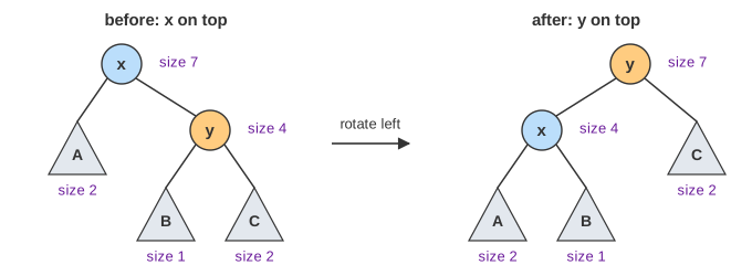
This page uses a plain, unbalanced BST so the walks are easy to follow, and refuses an insert that would go deeper than 6 levels. A real order-statistic tree is a red-black tree (as in CLRS) or an AVL tree with this extra field, so its height is O(log n) and every operation is too.
Running time
| operation | sorted array | balanced BST | order-statistic tree |
|---|---|---|---|
| search | O(log n) | O(log n) | O(log n) |
| insert / delete | O(n) | O(log n) | O(log n) |
| select(k) | O(1) | O(n), in-order walk | O(log n) |
| rank(key) | O(log n) | O(n) | O(log n) |
The extra cost is one integer per node. This is the textbook example of augmenting a data structure: a field that can be computed from a node's children alone can be kept up to date through inserts, deletes and rotations without changing their running time.
Where it is used
GCC's policy-based data structures ship one: __gnu_pbds::tree with tree_order_statistics_node_update gives find_by_order(k) (select) and order_of_key(x) (rank). Leaderboards and running medians use the same queries. Redis keeps the same counts in a different structure: each forward link of its skiplist stores a span, so ZRANK adds spans on the way down (see How a Redis Sorted Set Is Stored). A Fenwick tree answers rank over a fixed range of integer keys with prefix sums, and a treap or skip list can carry sizes the same way.
What the page leaves out
The tree holds at most 15 distinct keys on at most 6 levels and is never rebalanced; the rotations of a red-black or AVL tree are only described above. The page also leaves out duplicate keys (counted sizes per key), CLRS's bottom-up rank that walks from a node to the root with parent pointers, other augmentations such as interval trees (max endpoint per subtree), and counted B-trees used for positional access in databases and ropes.
See where this page fits on the Indexing mind map.