The idea: remember the biggest square that ends at each cell
You get a grid of 0s and 1s and want the largest square made only of 1s. Checking every top-left corner and every size works, but costs about R·C·min(R, C)² cell reads. Dynamic programming does it in one pass: for each cell, store the side of the largest all-1 square whose bottom-right corner is that cell.
The recurrence
Number rows and columns from 1 and give dp an extra row 0 and column 0 full of zeros, so every cell has three neighbours:
dp[i][j] = 0                                             if M[i][j] = 0
dp[i][j] = min(dp[i-1][j], dp[i][j-1], dp[i-1][j-1]) + 1   if M[i][j] = 1
answer   = (largest dp value)²                           the area
Each cell needs only the cell above (top), the cell to its left (left) and the diagonal (top-left), which are all filled earlier when you go row by row, left to right. In the animation the three neighbours turn blue, the smallest one darker blue, and the square the new value stands for is tinted green on the input matrix.
Why the minimum
A k×k square ending at (i, j) is the cell itself plus three overlapping (k−1)×(k−1) squares: one ending just above, one ending just to the left and one ending on the diagonal. All three must exist, so k − 1 can be at most the smallest of the three dp values. And when all three exist they cover every cell of the bigger square, so the bound is reached.
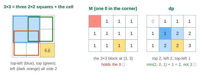
Taking the maximum, or only top and left, would be wrong. With a single 0 in the top-left corner, the cell at (3, 3) of 0111/1111/1111 has top 2 and left 2, but its top-left is 1, and indeed the 3×3 block ending there contains the 0 (Demo: one 0 in the corner). In the L-shape the arm cells have a big left and diagonal but a small top (Demo: L-shape).
Worked example
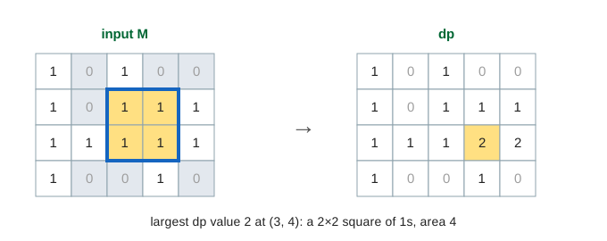
The LeetCode example (Demo: LeetCode 4×5 matrix):
M           dp
1 0 1 0 0   1 0 1 0 0
1 0 1 1 1   1 0 1 1 1
1 1 1 1 1   1 1 1 2 2     dp[3][4] = min(1, 1, 1) + 1 = 2
1 0 0 1 0   1 0 0 1 0     dp[3][5] = min(1, 2, 1) + 1 = 2
The largest value is 2, so the biggest square of 1s is 2×2, area 4. A matrix of all ones gives dp values that grow along each diagonal, up to the full size (Demo: all ones 4×4), and a matrix with a single 1 gives side 1 (Demo: a single 1).
Cost and the one-row version
| Method | Time | Extra space |
|---|---|---|
| Try every corner and size | O(R·C·min(R, C)²) | O(1) |
| dp table (this page) | O(R·C) | O(R·C) |
| dp, one row kept | O(R·C) | O(C) |
Each row of dp only reads the row above, so one array of length C + 1 is enough: before overwriting dp[j], save it, because it becomes the next cell's top-left.
Maximal rectangle: a different tool
The largest rectangle of 1s can't use this recurrence, because a rectangle ending at a cell has no single "size": a tall thin one and a short wide one don't compare. The standard method turns each row into a histogram: h[j] = how many 1s stand in a column ending at this row (reset to 0 at a 0). Then the largest rectangle in that histogram is found with a monotonic stack of bar indices in increasing height: when a lower bar arrives, pop the taller bars and measure the rectangle each one spans. That is O(C) per row, so O(R·C) in total, the same as the square.
Other grid DPs that fill a table from three neighbours: Edit Distance and Longest Common Subsequence. A table filled row by row with a traceback: 0/1 Knapsack.
What the page leaves out
Matrices are limited to 6 rows and 7 columns so both tables fit. The page does not animate the one-row version, counting all squares (the sum of all dp values), the maximal-rectangle histogram stack, or squares that may contain a few 0s.
See where this page fits on the Dynamic Programming mind map.