The idea: a line that gives probabilities
Logistic regression is a classifier for two classes, y = 1 or y = 0. Like the perceptron it draws a straight line through the inputs, but instead of a hard yes/no it gives a probability: points far on the class-1 side get p close to 1, points far on the other side get p close to 0, and points on the line get 0.5.
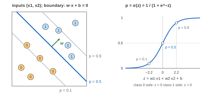
The page trains one on 10 points in the plane (or 12 that overlap), starting from a line that is the wrong way round, w = (1, −1), b = 0. Each panel shows one piece: the points and the line, the sigmoid with one dot per point, and the log loss of each point as a bar.
The sigmoid and the decision boundary
For a point x = (x1, x2) the model computes a score z = w1·x1 + w2·x2 + b and squashes it with the sigmoid σ(z) = 1 / (1 + e^−z) into p = P(y = 1 | x). σ(0) = 0.5, so the decision boundary p = 0.5 is exactly the line z = 0. The weight vector w is perpendicular to it and points toward class 1.
The lines p = 0.9 and p = 0.1 are z = ±ln 9 ≈ ±2.2. They sit at distance 2.2 / |w| from the boundary, so a longer w means a narrower band: |w| is how confident the model is, the direction of w is where the line points. (Demo: one point through the sigmoid.)
Log loss
A probability is judged by the log loss (cross-entropy) of the true class: −ln(p) when y = 1 and −ln(1 − p) when y = 0. The training loss L is the mean over all points. At the start, point 1 (class 1) gets p = 0.20, a loss of 1.61; point 2 (class 0) gets the same p = 0.20, but for it that is a good answer: loss 0.22.
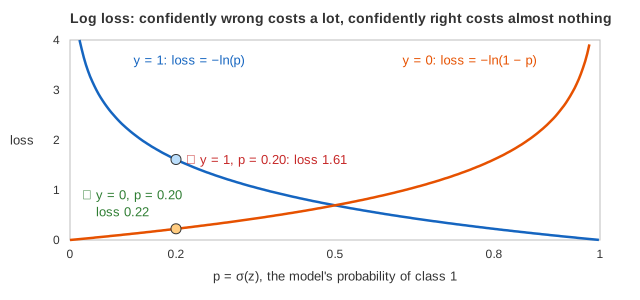
A model that says p = 0.01 for a point that is really class 1 pays −ln(0.01) = 4.6, so log loss punishes confident mistakes hard. It also comes from maximum likelihood: minimizing it is the same as making the observed labels as probable as possible.
The gradient: every point pushes by p − y
The derivative of the loss works out to something short:
- ∂L/∂w = mean((p − y)·x)
- ∂L/∂b = mean(p − y)
Each point pushes the weights by its error p − y times its input. One gradient descent step is w ← w − η·∇w, b ← b − η·∇b, and the line rotates and shifts. (Demo: one gradient step, narrated; Demo: train until every point is on its side.)
| Perceptron | Logistic regression | |
|---|---|---|
| output | a class ±1 (step) | a probability (sigmoid) |
| which points move the line | only mistakes | every point, by p − y |
| a point far on the right side | no effect | almost none (p − y ≈ 0) |
| overlapping classes | never settles | settles at the lowest loss |
Separable data: w keeps growing
When a line separates the classes, the loss can always get smaller by making w longer: every p moves closer to 0 or 1.
So L falls toward 0 but never reaches it, |w| grows without end, and the p = 0.1 / 0.9 lines close in on the boundary.
Real libraries stop this with regularization, a penalty λ·|w|² added to the loss (scikit-learn's
C = 1/λ). (Demo: separable data, w keeps growing.)
With overlapping classes no line gets every point right. The pushes of the misplaced points balance the others, w stops growing and L levels off above 0. (Demo: overlapping classes, the loss levels off.)
The learning rate
The log loss of logistic regression is convex: one bowl, no local minima, so gradient descent always heads to the same answer. η only sets the speed: after 20 steps η = 0.1 is still far from it while η = 2 is much closer. (Demo: learning rate 0.1 vs 2.) See Gradient Descent for steps that are too large and zig-zag.
Related models
| Model | Output | Loss |
|---|---|---|
| linear regression | a number w·x + b | mean squared error |
| logistic regression | p = σ(w·x + b) | log loss |
| softmax regression | one probability per class | cross-entropy |
| neural network | many logistic-like units in layers | log loss / cross-entropy |
See also Linear & Logistic Regression (the one-input version, where the sigmoid is drawn over x), Perceptron (the same line with a hard step and mistake-only updates), Gradient Descent, Softmax & Cross-Entropy for more than two classes, and Neural Network Forward Pass.
What the page leaves out
Only two inputs, so the boundary is a line you can see; with n inputs it is a hyperplane. Training is full-batch gradient descent with no regularization; real solvers (L-BFGS, Newton's method, liblinear) converge in far fewer steps and add an L2 penalty by default. Feature scaling, more than two classes (one-vs-rest, softmax), calibration, and non-linear boundaries from added features are not shown.