The idea: the average of many rolls settles down
Roll a fair die once and you get 1, 2, 3, 4, 5 or 6. Roll it ten thousand times and add up the rolls: the average is almost exactly 3.5. That number is the expected value E[X] of one roll, and the fact that the running average heads for it is the law of large numbers.
On the canvas the left panel lists the values of X with their probabilities (grey bars) and the share of the rolls so far (blue bars). The top right panel keeps the count n, the sum and the running average x̄ = sum / n. The chart plots x̄ against n on a log scale, with E[X] as a green line.
Expected value: a weighted average
For a random variable X with values x and probabilities P(x),
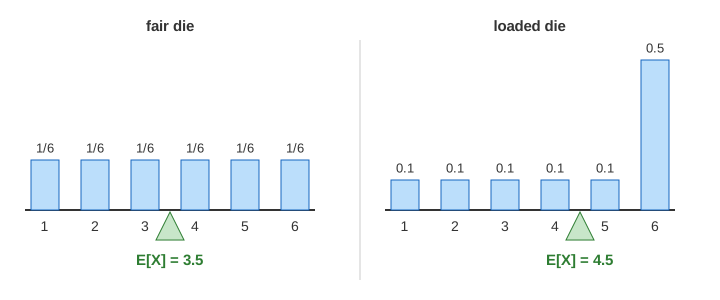
Each value counts as often as it is likely. For a fair die that is (1 + 2 + 3 + 4 + 5 + 6) / 6 = 21/6 = 3.5, a value no single roll can show. E[X] is not "the most likely roll"; it is what the rolls average out to. (Demo 1: E[X] of a fair die, term by term adds the six terms 0.167, 0.333, … one at a time.)
| Game | Values and P(x) | E[X] | σ (spread of one play) |
|---|---|---|---|
| fair die | 1 … 6, each 1/6 | 3.5 | 1.71 |
| loaded die | 1 … 5 each 0.1, 6 with 0.5 | 4.5 | 1.80 |
| bet | +10 with 0.3, −5 with 0.7 | −0.5 | 6.87 |
Expected value is linear: E[X + Y] = E[X] + E[Y] and E[aX] = a·E[X], even when X and Y depend on each other. So the expected sum of n rolls is n · 3.5, and the expected average is 3.5.
The law of large numbers
Roll independently, again and again, from the same distribution. The running average
The weak law says that for any margin, say 0.01, the chance that x̄ is more than 0.01 away from E[X] goes to 0 as n grows. The strong law says more: with probability 1, the sequence x̄₁, x̄₂, x̄₃, … itself converges to E[X]. The same law, applied to "did this roll show a 4?", says the share of 4s settles on 1/6: the blue bars creep up to the grey ones.
Seed 1 gives x̄ = 4.100 after 10 rolls, 3.360 after 100, 3.444 after 1000 and 3.486 after 10 000. (Demo 2: 10 rolls, one at a time and Demo 3: the running average to 10 000 rolls.)
How fast: σ/√n
The average of n independent rolls has standard deviation σ/√n, where σ is the spread of one roll (1.71 for a fair die). About 95% of runs stay inside E[X] ± 2σ/√n, the orange funnel. So 100 times more rolls make the typical error only 10 times smaller: 0.54 at n = 10, 0.054 at n = 1000, 0.017 at n = 10 000.
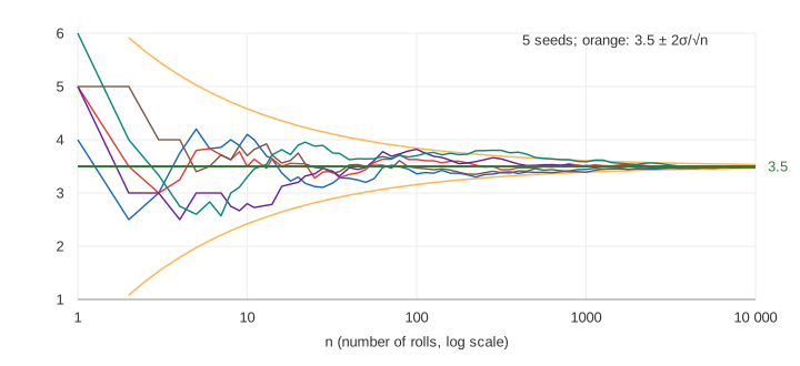
A different seed is a different experiment. Seed 2 ends at 3.506, seed 1 at 3.486; both are inside the funnel. (Demo 4: a different seed, same limit keeps seed 1's line in grey.) How the error is spread around E[X] (a bell curve) is the central limit theorem; the same 1/√n rule sets the accuracy of Monte Carlo estimates.
Diluted, not corrected
Suppose the first five rolls are all 6. The average is 6, and the sum is 30 − 5 · 3.5 = 12.5 above n · E[X]. Many people feel low numbers are now "due". They are not: a die has no memory, and each later roll is still 1 to 6 with 1/6 each. Believing otherwise is the gambler's fallacy.
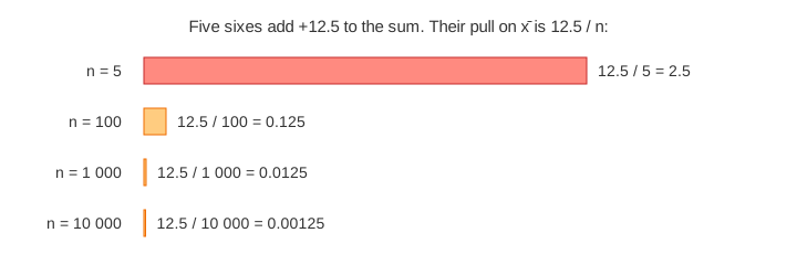
The average still goes to 3.5 because the 12.5 extra points are divided by an ever larger n. The gap sum − n · E[X] does not go back to 0; it keeps wandering, typically by about σ√n (171 at n = 10 000), in either direction. Only the gap divided by n shrinks. (Demo 5: five sixes are diluted, not corrected: x̄ = 5.100 after 10 rolls, 3.486 after 10 000, while the gap ends at −136.)
The house edge
A bet pays +10 with probability 0.3 and costs 5 with probability 0.7. E[X] = 3 − 3.5 = −0.5 per play. One play is a gamble (σ = 6.87, much bigger than 0.5), and after 100 plays seed 1 is even ahead (x̄ = +0.25). But after 10 000 plays the average is −0.489, and the total is about −4 900. A casino does not need luck: it needs E[X] < 0 for the player and many plays. Insurance works the same way from the other side. (Demo 6: a loaded die, E[X] = 4.5 ends at 4.492; Demo 7: a bet with E[X] = −0.5 ends at −0.489.)
See also mean vs median vs mode for the average of a fixed data set, and the Monty Hall problem, where 1000 simulated games settle on the 2/3 switching win rate.
What the page leaves out
Proofs (Chebyshev's inequality for the weak law, Borel–Cantelli for the strong law), variance as E[(X − E[X])²] in detail, distributions without a finite mean (the Cauchy distribution, where the running average never settles), continuous random variables and integrals, dependent samples (Markov chains have their own ergodic version of the law), and the large-deviation rate of how unlikely big errors are. The page stops at 10 000 rolls.
See where this page fits on the Probability & Statistics mind map.