Interpolation vs Splines Visualization

The idea: a curve through the dots

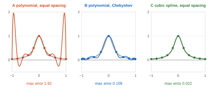
You know a function only at a few points, from a measurement, a table or an expensive computation, and you want values in between. Interpolation draws a curve that passes exactly through every known point. The page compares three ways to do it on the same function, side by side: one polynomial through equally spaced points (panel A), one polynomial through Chebyshev points (panel B), and a cubic spline through the equally spaced points of A (panel C).

Runge's function with 11 points: the same data three ways, max errors 1.92, 0.109 and 0.022.

One polynomial through n points

Through n points with different x values there is exactly one polynomial of degree at most n − 1. The Lagrange form writes it down directly:

p(x) = y₀·ℓ₀(x) + y₁·ℓ₁(x) + … + y_n−1·ℓ_n−1(x), ℓ_i(x) = ∏_j≠i (x − x_j)/(x_i − x_j)

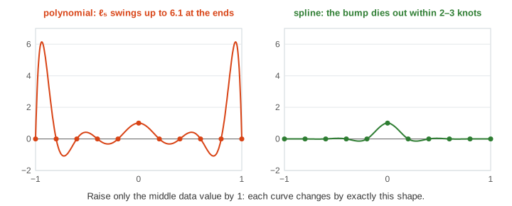
Each basis polynomial ℓ_i is 1 at its own node and 0 at all the others, so the sum hits every y_i. Between the nodes, though, ℓ_i is free to swing. The page evaluates p with the barycentric form of the same formula, which is fast and numerically stable. The same idea, over a finite field, rebuilds lost data in Reed-Solomon codes. (Demo: Lagrange basis, why the ends swing)

Runge's phenomenon

Carl Runge noticed in 1901 that for f(x) = 1/(1 + 25x²) on [−1, 1], more equally spaced points make the polynomial worse. The middle gets better, but near the ends the curve swings harder with every new point:

n points	equally spaced	Chebyshev	cubic spline
5	0.438	0.402	0.279
9	1.05	0.171	0.0561
11	1.92	0.109	0.0220
13	3.66	0.0692	0.00691
17	14.4	0.0326	0.00375
21	✗ 59.8	✓ 0.0153	✓ 0.00318

The error formula explains it: f(x) − p(x) = f⁽ⁿ⁾(ξ)/n! · (x − x₀)(x − x₁)…(x − x_n−1). For equally spaced nodes the product is tiny in the middle and huge near the ends, and for Runge's function the derivatives f⁽ⁿ⁾ grow even faster than n!. The function is smooth on the real line, but its Taylor series around 0 only converges for |x| < 0.2, because of poles at x = ±0.2i. (Demo: Runge, more points make it worse; Demo: error table for Runge's function)

Chebyshev points

The fix that keeps one polynomial is to move the points. Chebyshev points x_k = cos((2k + 1)π / 2n) are equally spaced angles on a half circle, dropped onto the axis. They crowd toward the ends, exactly where the equally spaced product was large, and they make the product (x − x₀)…(x − x_n−1) as small as it can be: at most 2¹⁻ⁿ everywhere on [−1, 1].

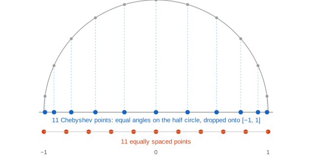
Chebyshev points are the shadows of equally spaced points on a half circle: dense at the ends.

With these nodes every basis polynomial stays small (for n = 11, |ℓ_i| ≤ 1.27 against 6.5 on equal spacing), and for Runge's function the error falls steadily: 0.109 at n = 11, 0.0153 at n = 21. The catch: you must be able to choose where to sample. Measured data usually comes on a fixed grid.

Cubic splines

A cubic spline gives up the single formula. It uses one cubic piece per gap between two neighbouring points, and joins the pieces so that the value, the slope and the curvature (second derivative) match at every inner point, the knots. That leaves two conditions free; the natural spline used here sets the curvature to 0 at both ends. Finding the curvatures M_i at the knots is one tridiagonal linear system, solved in O(n) steps. Because each piece has degree 3, there is nothing to swing: the error falls like h⁴ with the gap h, on the same equally spaced points that defeat the polynomial. Piecewise cubic curves are also how drawing programs and fonts work; see Bézier curves.

Global vs local

Change one data value and see what moves. Every method here is linear in the data, so raising y_i by d adds d times that node's basis curve. A polynomial's basis curves cover the whole interval: raise the middle point of 11 equally spaced points and the curve jumps by up to 3 near the ends. A spline's basis curve is a bump that dies out within two or three knots. (Demo: move one point, global vs local)

Left: the polynomial basis function for the middle of 11 equally spaced nodes, 1 at x = 0 and 0 at the other nodes, swinging up to 6.1 near x = ±0.95. Right: the cubic spline basis function for the same node, a bump at 0 with small ripples that vanish within two or three knots. — The middle node's basis curve: the polynomial's reaches across the whole interval, the spline's stays local.

Which one to use

situation	good choice	why
data on a fixed grid, many points	cubic spline	no swings, local, O(n) to build
you choose the points, f very smooth	polynomial on Chebyshev points	error falls faster than any power of 1/n
a few points (n ≤ 5)	any of them	low degree cannot swing much
noisy data	none: fit, don't interpolate	passing through every point copies the noise

No method always wins. For the smooth sin(πx), the polynomials reach 10⁻¹³ at n = 21 while the spline stops near 3·10⁻⁵ (Demo: smooth sin(πx), the polynomials win). For |x|, with a corner at 0, the polynomial on equal spacing blows up and the spline does best (Demo: a kink |x|, the spline wins). For noisy measurements a curve that passes near the points is better than one through them; see least squares.

What the page leaves out

Other end conditions for splines (clamped, with given end slopes, and not-a-knot, the default of scipy.interpolate.CubicSpline), shape-preserving piecewise cubics (PCHIP, Akima) that avoid overshoot, B-spline bases, Hermite interpolation that also matches slopes, Newton's divided-difference form, the Lebesgue constant that measures how much a node set can amplify errors, rounding error in the monomial form, and interpolation in 2D or more.