The idea: tidy up now, or tidy up later
Both are priority queues: they hand back the smallest key first. Both support insert, extract-min and decrease-key (make a key smaller, as Dijkstra's algorithm does when it finds a shorter path). The page gives the same operations to a binary heap (left) and a Fibonacci heap (right) and counts the work each one does. One step on the canvas is one piece of work in each heap, so the heap with less to do finishes first and shows ✓.
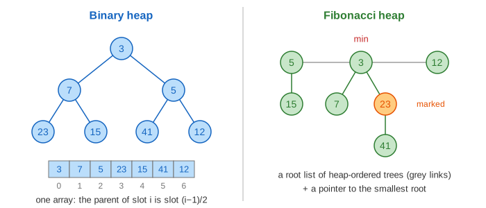
The binary heap keeps its shape exact after every operation. The Fibonacci heap does as little as it can and leaves the mess for later. The mess is paid for in extract-min, which links trees together until they are tidy again.
Binary heap: tidy after every operation
- Insert: write the key into the next free array slot, then sift it up: compare with the parent, swap while smaller. At most log₂n swaps.
- Extract-min: take slot 0, move the last key there, then sift it down: compare the two children, swap with the smaller while it is smaller. About 2 log₂n comparisons.
- Decrease-key: lower the key in place, then sift it up, like an insert.
Every operation is O(log n) in the worst case, and the work never builds up.
Fibonacci heap: lazy until extract-min
- Insert: add a one-node tree to the root list and compare it with the min. Two units of work, whatever n is (Demo: 15 inserts).
- Extract-min: remove the min root; its children join the root list. Then consolidate: walk the roots with a degree table A[d] and link any two trees of the same degree (the larger root goes under the smaller) until no two roots have the same degree. Finally scan the roots for the new min.
- Decrease-key: lower the key. If it is now smaller than its parent, cut it off and make it a root. A parent that loses its first child is marked; a marked parent that loses a second child is cut too, and so on up (cascading cut). The marks keep every tree bushy enough that a root of degree d has at least Fd+2 nodes (a Fibonacci number, hence the name), so degrees stay below about 1.44 log₂n.
How the page counts work
Work = comparisons + moves. A move is one array write or swap, one root added to the root list or the degree table, one link, one cut, or one mark. The scoreboard shows, for each heap, the work of the current operation, the total, the average per operation and the most work any single operation took. Numbers like these hide constant factors (a Fibonacci node holds four pointers, a degree and a mark; a binary heap node is one array slot), so read them as a picture of the shape of the cost, not a benchmark.
Amortized vs worst case
After 15 inserts the Fibonacci heap has done 29 units of work to the binary heap's 49, but it is just a list of 15 roots. The first extract-min pays for that: it links the 14 remaining roots into 3 trees and costs 39 units, against 9 for the binary heap (Demo: inserts, then 3 extract-mins). The next two extract-mins cost the Fibonacci heap 11 and 16, close to the binary heap's 10 and 10.
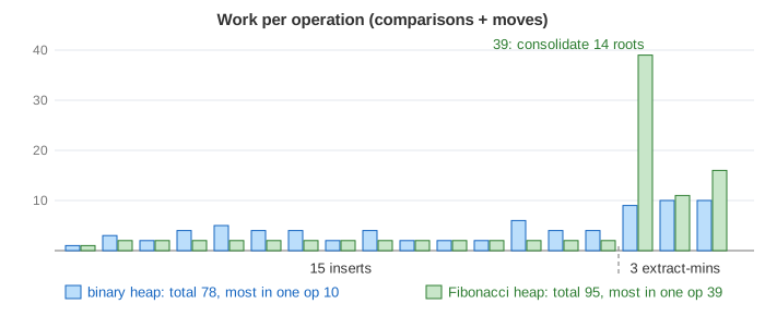
This is what amortized cost means. Give the heap a potential Φ = roots + 2 · marked nodes (the Fibonacci stats line shows it). Each insert raises Φ by 1, and that stored-up credit pays for the links later; an extract-min that does a lot of linking also lowers Φ a lot. Counted this way, insert and decrease-key cost O(1) and extract-min O(log n), averaged over any sequence of operations. A single extract-min can still cost O(n), which the "most in one op" number shows. A binary heap never has such spikes.
Decrease-key and cascading cuts
Lowering a deep key in a binary heap means sifting it up level by level. Demo: a decrease-key burst lowers five keys on the bottom level to new minimums: each one climbs 3 levels, 7 units of work each, 35 in all. The Fibonacci heap cuts each key off in one move and spends 4 or 5 units per decrease-key, 23 in all. That is the O(log n) vs O(1) difference.
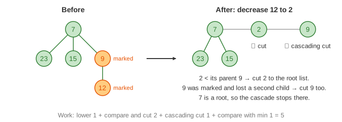
The cuts are not free in the long run. Every cut adds a root, and the next extract-min must link it back in. In Demo: cascading cut three decrease-keys (the last one with a cascading cut) cost the Fibonacci heap 15 and the binary heap 19, but the extract-min that follows costs the Fibonacci heap 15 and the binary heap 7, so the binary heap ends ahead, 26 vs 30.
Dijkstra: where the O(1) decrease-key should pay off
Dijkstra's algorithm on n vertices and m edges does n inserts, n extract-mins and up to m decrease-keys. With a binary heap that is O((n + m) log n); with a Fibonacci heap O(m + n log n), the best bound known for this algorithm and the reason Fibonacci heaps were invented (Fredman and Tarjan, 1984). Demo: Dijkstra, 8 vertices runs it on a small graph (A to H, 14 edges, 13 decrease-keys): the binary heap does 72 units of work, the Fibonacci heap 108. Measured with this page's own code on bigger graphs (random edge weights 1–100):
graph                              decrease-keys   binary heap   Fibonacci heap
8 vertices, 14 edges (the demo)         13              72            108
100 vertices, 500 random edges         136           2,215          3,322
1,000 vertices, 5,000 random edges    1,330          32,429         49,736
1,000 vertices, 100,000 random edges  1,452          32,392         50,697
1,000 vertices, every pair (worst)  499,500       1,023,283      1,522,984
The binary heap wins every row. On random graphs few edges lead to a decrease-key (about n ln(m/n)), so the extract-mins dominate, and a binary heap's extract-min is cheaper. Even when almost every edge is a decrease-key (the last row), the lowered keys rarely climb more than a level or two in the binary heap, so its "O(log n)" decrease-key costs about 2 units in practice. The Fibonacci heap's advantage is a guarantee about the worst case of very large, very dense graphs; on real inputs the binary heap is faster.
When to pick which
| Binary heap | Fibonacci heap | |
|---|---|---|
| insert | O(log n) | O(1) |
| extract-min | O(log n) | O(log n) amortized, O(n) worst single op |
| decrease-key | O(log n) | O(1) amortized |
| merge two heaps | O(n) | O(1): join the root lists |
| memory | one array, no pointers | 4 pointers + degree + mark per node |
| pick it for | almost everything: schedulers, timers, Dijkstra and A* in practice, heap sort | proofs of running time; very dense graphs; when every operation's average matters more than its worst case |
Most standard libraries (Java's PriorityQueue, C++'s std::priority_queue, Python's heapq) are binary heaps, and many skip decrease-key entirely: Dijkstra just inserts the vertex again and skips stale entries when they come out. See also Priority Queues (binary heap) and Binomial Queues, whose linking step is the one Fibonacci heaps use.
What the page leaves out
The heaps hold at most 15 distinct keys, and work is counted in operations, not measured in time; real costs also depend on cache misses and memory allocation, where the array-based binary heap is far ahead. The page leaves out delete (decrease-key to −∞, then extract-min), merging two heaps, d-ary heaps (wider nodes, fewer levels, faster decrease-key), pairing heaps (simpler, often the fastest in practice) and other variants such as rank-pairing and strict Fibonacci heaps, which keep the same bounds with less overhead or without amortization.