The idea: count operations, not seconds
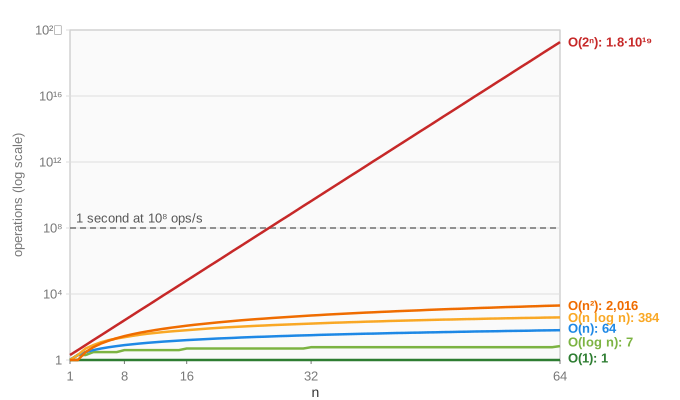
Big-O describes how the number of basic operations an algorithm makes grows with the input size n. Seconds depend on the machine; the count does not. The page runs six real algorithms on the same sorted array of n values. Each one counts its own basic operation, and a bar shows the count on a log scale: every 4 marks on the axis is 10,000 times more work.
The six rows
| Row | Algorithm | One operation is | Count |
|---|---|---|---|
| O(1) | read a[5] | one array read | 1 |
| O(log n) | binary search for a key bigger than every value (3n + 5, the worst case) | one probe of a[mid] | ⌊log₂ n⌋ + 1 |
| O(n) | linear scan for the same key | one comparison | n |
| O(n log n) | top-down merge sort | one value written by a merge | about n·log₂ n (exactly n·log₂ n when n is a power of 2) |
| O(n²) | bubble sort without the early exit | one comparison | n(n−1)/2 |
| O(2ⁿ) | check every subset: does it add up to the key? | one subset checked | 2ⁿ |
A row says counted when the page actually ran the code with a counter (up to a million operations), and formula when it would take too long, as bubble sort on a million values would. Where both exist they agree. Press Trace (for n up to 32) to watch the first few operations of each algorithm on the drawn array (Demo: n = 8, everything is fast).
What doubling n does
The quickest way to feel a growth rate is to double n and see what happens to the count (Demo: doubling n):
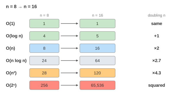
O(n log n) grows a little faster than ×2 because each value also passes through one more level of merging. O(n²) tends to ×4 (28 → 120 is ×4.3 because of the −1). O(2ⁿ) is squared: 2¹⁶ = (2⁸)².
From operations to time
The page assumes 10⁸ simple operations per second, about 10 ns each, which is the right order for a simple loop on one core. At n = 1000, bubble sort's 499,500 comparisons take 5 ms and merge sort’s 9,976 writes take 100 µs: 50× apart, and the gap grows with n. At a million values it is 1.4 hours against 0.2 seconds (Demo: n = 1000, n² vs n log n).
| n | 2ⁿ subsets | time at 10⁸ ops/s |
|---|---|---|
| 8 | 256 | 2.6 µs |
| 16 | 65,536 | 660 µs |
| 32 | 4,294,967,296 | 43 s |
| 64 | 1.8·10¹⁹ | ≈ 5,800 years |
| 1000 | 1.1·10³⁰¹ | 3.4·10²⁸⁵ years |
A faster computer does not rescue an exponential algorithm: a machine 1,000 times faster only moves the 1-second point from n ≈ 27 to n ≈ 37 (Demo: 2ⁿ blows up).
Constants matter at small n
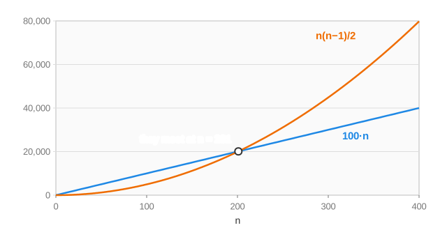
Big-O drops constant factors. Set O(n) cost to 100 operations per item (parsing, hashing, a cache miss) and the linear row becomes 100·n. At n = 8 that is 800 operations against bubble sort's 28, and at n = 32 it is 3,200 against 496: the "worse" algorithm wins. They meet at n = 201. At n = 1000 the linear scan is ahead 5×, and from there it only gets further ahead (Demo: constants matter). This is why real sorts switch to insertion sort for short ranges.
See the Sieve of Eratosthenes for n·ln ln n work against trial division's n√n / ln n on real counts.
Why log n grows so slowly and 2ⁿ so fast, with log₂ as the mirror image of 2ˣ: see Exponentials and Logarithms.
What the page leaves out
Real running time also depends on memory access, caches and branch prediction, so one "operation" is not always 10 ns. Big-O is an upper bound; the page shows exact counts for one input, and binary search and linear scan are shown in their worst case. Average-case and amortized analysis, Θ and Ω, and space complexity are not drawn. See also Sorting Race (two sorts side by side on the same array), Binary and Linear Search and Comparison Sorting.